Can you use standard deviation in project management?

Standard deviation is an abstract concept derived from observation rather than calculation or experimentation. The standard deviation (SD, also represented by the Greek letter sigma or σ) is a measure that is used to quantify the amount of variation or dispersion in a set of data values. It is expressed as a quantity defining how much the members of a group differ from the mean value for the group.

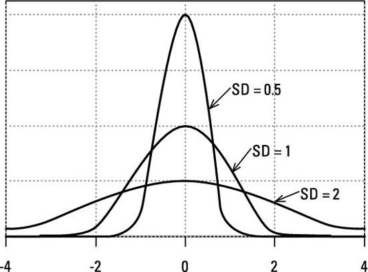
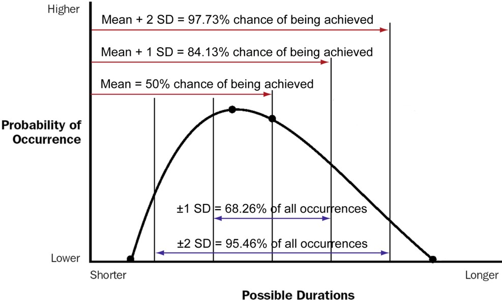
A low value for the standard deviation indicates that the data points tend to be close to the mean or the expected value of the set, while a high value indicates that the data points are spread out over a wider range. The area under each of the three curves in the diagram below are the same, representing the same population. The values could be millimetres or days depending on what’s being measured: where the SD is small, at 0.5, everything is clustered close to the mean, some 98% of all of the values will be in the range of +2 to -2. Where the SD is large, at 2.0, a much larger number of measurements are outside of the +2 to -2 range.

The concept of SD and ‘normal distributions’ is part of the overall concept of probability and understanding the extent to which the past can be relied on to predict the future. The future is, of course, unknown (and unknowable) but we have learned that in many situations what has happened in the past is of value in predicting the future. The key question is: to what degree should we rely on patterns from the past to predict the future?

Applications of standard deviation

The journey towards understanding probability started in 1654 when French mathematicians Blaise Pascal and Pierre de Fermat solved a puzzle that had plagued gamblers for more than 200 years: how to divide the stakes in an unfinished game of chance if one of the players is ahead? Their solution meant that people could for the first time make decisions and forecast the future based on numbers.

Over the next century, mathematicians developed quantitative techniques for risk management that transformed probability theory into a powerful instrument for organising, interpreting and applying information to help make decisions about the future. The concepts of Standard Deviation and ‘Normal Distribution’ were central to these developments.

Understanding populations became the ‘hot topic’, and by 1725 mathematicians were competing with each other to devise tables of life expectancy, as the UK government was financing itself through he sale of annuities, and tables to facilitate setting marine insurance premiums, to name a few uses.

Some of the phenomena studied included the age people died at, and the number of bees on a honeycomb and based on many hundreds of data sets the observation that natural populations seemed to have a ‘normal’ distribution started to emerge. In 1730 Abraham de Moivre suggested the structure of this normal distribution, the ‘bell curve’, and discovered the concept of the Standard Deviation. Advancing this work involved many famous mathematicians, including Carl Friedrich Gauss. One of the outcomes from Gauss’ work was validating de Moivre’s ‘bell curve’ and developing the mathematics needed to apply the concept to risk.

I will not deal with the calculation of a standard deviation here as the process is horrible. But we will look at how the concepts can be applied.

As we go forward, the important thing to remember is that every process and every population has a degree of randomness. This normal variation may be large or small depending on the process or the population and the normal distribution curve defined by its standard deviation provide tools to help understand the probable range of outcomes we can expect.

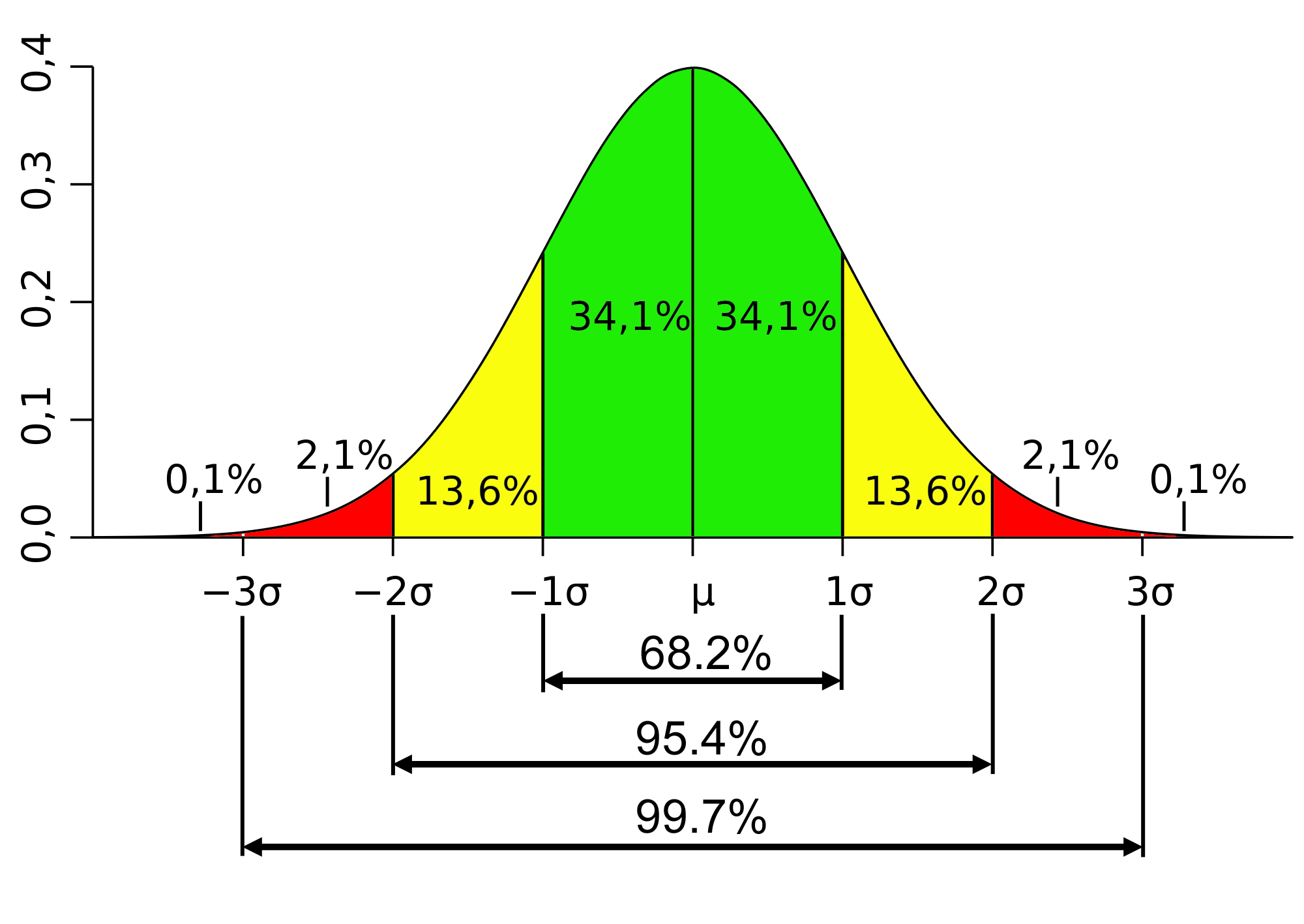
This prediction is not certain, but there is a high degree of probability the prediction will be reasonably correct, and the degree of certainty increases as the amount of data used in the analysis increases. The other key outcome from Gauss’ work was the finding that the percentage of the population occurring close to the mean and further from the mean followed a consistent pattern, with up to 99.99% occurring within ±6 standard deviations (σ) provided the distribution was ‘normal’.

How to use deviations in project management

The first major challenge in understanding the concept of a standard deviation is to appreciate it was derived from looking at data obtained from 100s of measurements of a natural phenomenon. Therefore these functions will have less value in determining the consequences of a one-off uncertainty such as a unique project outcome or a single risk event—but they are still useful.

For every population being measured, the key things to remember are:

• The SD is expressed in the same terms as the factor being measured. If the factor being measured is the age people die at, expressed in years, the SD will be measured in years (important for annuities and life insurance); if the factor being measured is the length of a bolt expresses in millimetres, the SD will be expressed in millimetres.
• The value of the SD for a specific population is constant, if 1 SD = 0.5mm, 2 SD = 1mm and 6 SD = 3mm, therefore if the target length for the bolt is 100mm and the mean (average length) produced is also 100mm 99.99% of the bolts manufactured will be between 97mm and 103mm in length (±6 SD).
• The percentages for 1 SD, 2 SD, 3 SD and 6 SD are always the same because the value of the SD expressed in millimetre, years, and so on, varies depending on the overall variability of the population, and of course the factor being measured.

How this plays out in the real world depends on circumstances. Staying with bolts, they are designed to fasten two things together and therefore need to be a minimum length. If your require bolts with a minimum length and want at least a 99.99% certainty every bolt will pass the test, with an SD of 0.5mm the manufacturer will need to set the manufactured length to 103mm. 99.99% of the bolts will then be in the range 100mm to 106mm (±6 SD). Only 1 in 10,000 will fall outside of this range and only 1 in 20,000 will be short—the other half will be slightly longer than 106mm.

If you can accept a slightly larger number of errors, you could adjust the requirement to ±3 SD. Now the manufacturer can set the manufactured length to 101.5mm. 99.7% of the bolts will be in the range of 100mm to 103mm and 3 in a thousand will be a bit longer or shorter – therefore by accepting 1.5 bolts in a thousand may be too short, the manufacturer can save 1.5mm of steel per bolt = 1.5 metres for every 1,000 bolts manufactured as the reject length is 1.5 * 100mm – 150mm of stock plus manufacturing costs. This should be a significant cost saving for a slightly increased defect rate.

Now assume a new manufacturer sets up in the bolt business, with new machinery that is more precise in its operation. This manufacturer can produce bolts with a SD of 0.1mm. Therefore it can deliver bolts with a 99.99% probability of every bolt being at least 100mm long with a target manufacturing length of 100.6mm! The ±6 SD range is now from 100mm to 101.2mm. The higher precision in the manufacturing process produces materials savings and a more consisted success rate with only 1 in 20,000 bolts likely to be too short.

How does this apply to projects?

When we start using standard deviation in project management there are a number of logical issues. For most factors involved in the overall project, we are confronted by the problem that every project is unique, that is, the population is ‘1’ and therefore the data needed to correctly estimate a SD is never going to be available, though obviously this does not apply to mass produced components used within the project such as bolts.

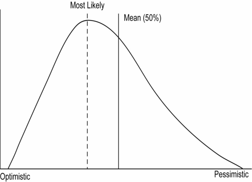
The second major issue is the distribution of project outcomes tends to follow a beta distribution rather than a balanced ‘normal’ distribution because, generally, the number of things that can go wrong on a project are far greater than the number of things that can go right.

The consequence is the average value (mean) is moved away from the most likely value, this significantly devalues the reliability of the SD concept:

Finally, in many situations the objective is not ‘plus or minus’ but rather focused on achieving an objective. No one ever got fired for coming in under budget. This changes the model significantly:

The concept of standard deviation can still be used, but the reliability is significantly reduced. These problems are discussed in Understanding PERT.

The difficulty in predicting the probability of completing a project by a certain date or for a certain price has been solved by applying the power of modern computers. Monte Carlo does not assume any range of outcomes, it uses brute force to calculate hundreds of different outcomes and then plots the results:

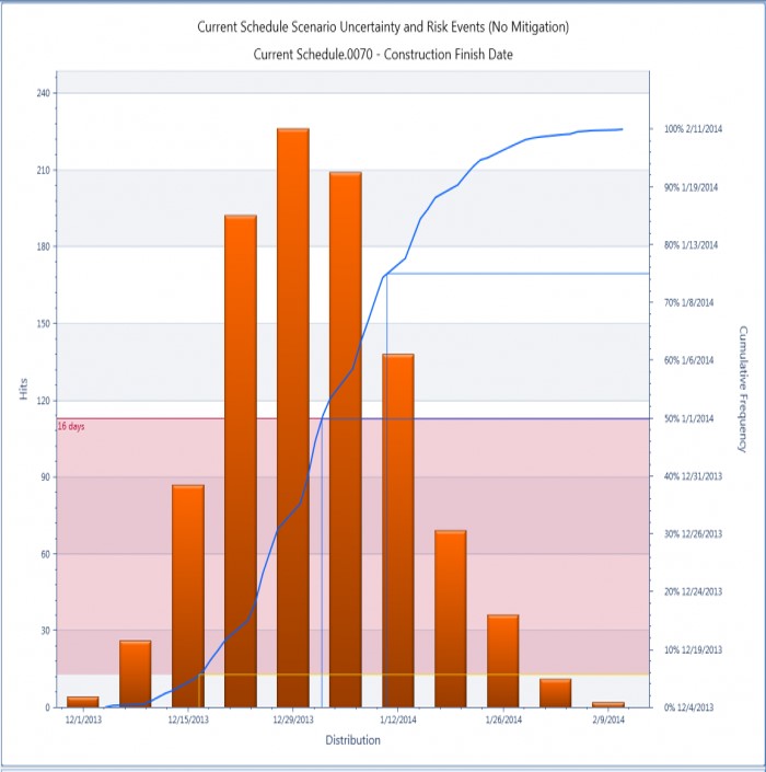
The resulting plot can be used to assess probability but it is based on hard data, not an assumed standard distribution.

The concept of standard deviation and normal distributions are valuable quality control tools where the project is making or buying hundreds of similar components. It is less valuable in dealing with the probability of completing a one-off ‘unique’ project within time or budget. In both situations, understanding variability and probability is important, but faced with the uncertainties of a ‘unique project’ Monte Carlo provides a more reliable approach.