On probability, randomness and risk

Does the result of the Rugby League Grand Final this recent weekend prove that the North Queensland Cowboys are a better team than the Broncos? Maybe not! The central claim in The Drunkard’s Walk by Leonard Mlodinow is that most people cannot predict the probability of anything: in all probability, we all get the probability wrong!

There are three basic laws of probability:

1. The probability that two events will occur can never be greater than the probability that each will occur individually.
2. If two events A and B to are independent, the probability that both A and B will occur is the product of their individual probabilities.
3. If an event can have a number of distinct and different outcomes, A, B, C, etc, the probability that either A or B will occur is equal to the sum of the individual probabilities of A or B occurring and the sum of all of the probabilities equals 1 (ie, there is a 100% probability that one of the options will occur).

In summary, if you want to know the probability that both A and B will occur you multiply; if you want to know the probability of whether A or B will occur you add. We will get to each of these in due course. But first we need to understand where probability occurs±—this is called the sample space.

Sample space

The first step to understanding probability is understanding the ‘sample space’, this ‘space’ represents the range of options, that is possible outcomes, from any given situation.

The Australian game of Two-up involves tossing two coins simultaneously from a wooden ‘kip’ the outcome can be 2, 1 or 0 heads ‘up’ (showing). What are the chances of tossing with the coins landing two heads up?

Despite there only being three possible outcomes, the answer is not 1/3, because the sample space is bigger than the three outcomes and depends on the sequence of the coins showing H for heads or T for tails. The possible options are: HH, HT, TH, TT.

There are 4 possible outcomes, giving a 25% probability of any one toss returning two heads. Similarly there is a 50% probability of a toss producing one head, and a 75% probability of a toss producing at least one head (that is, one or two) showing.

The concept of the ‘sample space’ was generalised by Gerolamo Cardano in 1520 but was not published for another 100 years, in 1663. The general rule is ‘suppose a random process has many equally likely outcomes, some favourable others unfavourable, then the probability of obtaining a favourable outcome is equal to the proportion of outcomes that are favourable’. The set of all possible outcomes is called the sample space.

Sequence matters

Within a sample space, the sequence matters! Instead of coins, let’s consider a mother carrying a set of fraternal twins. The options are girl-girl, girl-boy, boy-girl or boy-boy. If the mother knows one of the twins is a girl, what is the probability of having two girls?

Our knowledge of the ‘sample space’ eliminates the B-B option leaving three possibilities, one of which is G-G, a probability of 33.33%. However, if we know the first twin is a girl, we can eliminate two possibilities, the B-B and the B-G options. Now there are only two options left and the likelihood of the G-G option increases to 50%.

Which brings us to the classic ‘pick-a-box’ problem, also known as the Monty Hall problem, based on an American game show, Let’s Make a Deal. (This almost always ends up in an argument in our PMP class.) At the finale of each show, the winner is presented with three boxes, one of which contains a valuable prize. The contestant has to select one box. Before opening the selected box, the host opens one of the other two, being careful to select an empty box. The contestant is then offered the opportunity to change boxes—what should s/he do?

Using the concept of a sample space, there is a 33.33% probability of the prize being in any one of the boxes, and therefore a 66.66% probability the contestant has made the wrong choice. The fact that the show host has proved the obvious, one his boxes had to be empty, does not change the situation. The contestant still has a 33.33% chance of having made the winning choice and a 66.66% chance of having made a losing choice, the best choice is to make the swap.

Decades of game show results confirm that people who made the swap on average were twice as successful as those who chose to stay with their original choice. The situation does not change if the host is unaware of the box’s contents. The only difference would be on about 33.33% of the plays, the host would open the winning box and spoil the show—on the other occasions the odds are still 2:1 in favour of swapping.

Pascal’s triangle

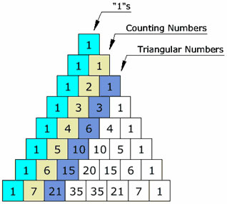
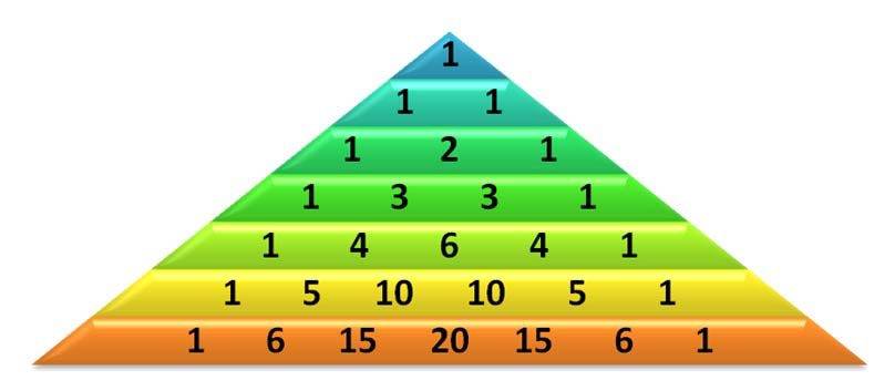
The next major development in the concept of the ‘sample space’ is called Pascal’s triangle. The computational method was developed by Chinese mathematician Jia Xain around 1050 and published by Zhu Shijie in 1303 and discussed in a work by Cardano published in 1570 before being picked up by Blaise Pascal, although but Pascal’s name predominates.

The triangle is constructed by adding the two numbers in the line above to the left and right of the new line (add 0 if there is no number). The first number in each line is the number of ways you can select a group of zero from the available options (there is only ever one way to select nothing).

The second number is the number of ways you can group individual members and is also the line number you can select 1 once, 2 once, etc. The third number is the possible ways to select groupings of 2, and so on.

Why this matters can be demonstrated by a small focus group of six people brought together from a larger population to assess a new product. If the overall population are split 50% for the product and 50% against, what is the probability of the sample group providing you with a correct 50/50 a split?

Using Pascal’s triangle we can see on line 6 the possible groupings of 0 people, 2 people, 3, 4, 5 or 6 people that like your product. There:

• is only 1 option that no one likes it;
• are 6 options that 1 person likes it (the ‘counting’ number);
• are 15 options (ie, possible different groupings) that 2 people like it;
• are 20 options that 3 people like it (1, 2 & 3; 1, 2 & 4, 1, 2 & 5, 1, 2 & 6; 1, 3 & 4; etc);
• are 15 options that 4 people like it;
• are 6 options that 4 people like it; and to finish
• only 1 option that all 6 people like it

In total, the ‘sample space’ has 64 options (1+6+15+20+15+6+1), and there are only 20 ways the group could split 50/50. This means there is:

• a 20/64 probability (roughly 30%) of getting the correct answer; and
• 44 ways (1+6+15+15+6+1) (roughly 70%) probability you could get a misleading result, and this assumes there is a truly random selection of people in the focus group.

The same principles apply to competitive situations; the best players don’t always win. If the two finalists at the Australian open are equally matched, there is of course a 50/50 probability of either winning. However, if the better player has a 55% to 45% advantage over the second ranked player the #2 player can expect to win a five-set match around 40% of the time. You would need a series of more than 250 games to be statistically certain, that is with an error of less than 5%, that the best player had actually won the championship.

So if anyone from Townsville is reading this, the Cowboys may be the better team or their win over the Broncos may simply be due to the probability and randomness, but after 20 years of trying, mathematics won’t stop the party.

This is the first of three articles based on Leonard Mlodinow’s book, The Drunkard’s Walk. In the next article we will look at randomness, and then finally how this affects everything in project controls and business.